Double Descent Part I: Sample-wise Non-monotonicity
One of the most fascinating findings in the statistical/machine learning literature of the last 10 years is the phenomenon called double descent. For some reason, extremely over-parameterized models, where the number of parameters to estimate is 10-1000 times more than the number of observations, sometimes win competitions, prove to be the best models. How can this be in the presence of the bias-variance trade-off? How come the variance does not become enormous in these models? One explanation is that the U-shaped bias-variance trade-off curve takes a second downward turn at the end of the U, hence the name double descent. It’s almost magical. It’s almost like we pass through a portal, and in the new bizarro universe, the gravity pushes.
Today, we will briefly talk about the idea behind the second descent and show its existence. In particular, we will see what happens when we know the functional form of the underlying data generating process, but we have small number of observations. This is one of the cases where double descent can occur, and it is called sample-wise double descent.
Bias-Variance Trade-off and Different Parameterization Regimes
Bias-variance trade-off is one of the most basic concepts that pretty much everybody doing prediction/forecasting should know. Briefly, it is saying that very simple models produce predictions with high bias and low variance, and as we construct more complex models to decrease the bias, we tend to increase the variance. At a certain point, the decline in bias is too small compared to the increase in the variance. Since the prediction error depends on both of them (for instance, \(MSPE = Variance + Bias^{2}\)), we need to find the sweet spot where neither the bias nor the variance is minimized, but both are small enough. In Figure 1, it is shown as the black point on the “Variance + Bias\(^2\)” curve. It is the point where the prediction error is minimized.1
library(tidyverse)
#Prediction error
f <- function(x){
  (-0.4 + 1/(x+0.5)) + (0.5*exp(x))
}
#The point where the prediction error is minimized
optimum <- optimize(f, interval=c(0, 1), maximum=FALSE, tol = 1e-8)
temp_data <- data.frame(x = optimum$minimum, y=optimum$objective)

ggplot(data = temp_data, aes(x=x, y=y)) +
  xlim(0,1) +
  geom_function(fun = function(x) 0.5*exp(x), color = "red", size = 2, alpha = 0.7) +
  geom_function(fun = function(x) -0.4 + 1/(x+0.5), color = "blue", size = 2, alpha = 0.7)  +
  geom_function(fun = function(x) (-0.4 + 1/(x+0.5)) + (0.5*exp(x)), color = "forestgreen", size = 2, alpha = 0.7)  +
  geom_point(size =3) +
  theme_minimal() + ylab("Error") + xlab("Model Complexity") +
  theme(axis.text=element_blank(),
        axis.ticks=element_blank()) +
  annotate("text", x=0.2, y=0.11+1/(0.2+0.5)-0.35, label= expression(paste("B", ias^2)), color = "blue", size =5) +
  annotate("text", x=0.2, y=0.11+0.5*exp(0.2), label= "Variance", color = "red", size =5) +
  annotate("text", x=0.32, y=-0.35+ 0.11+(0.5*exp(0.2) + 1/(0.2+0.5)), label= expression(paste("MSE = Variance + B", ias^2)), color = "forestgreen", size =5)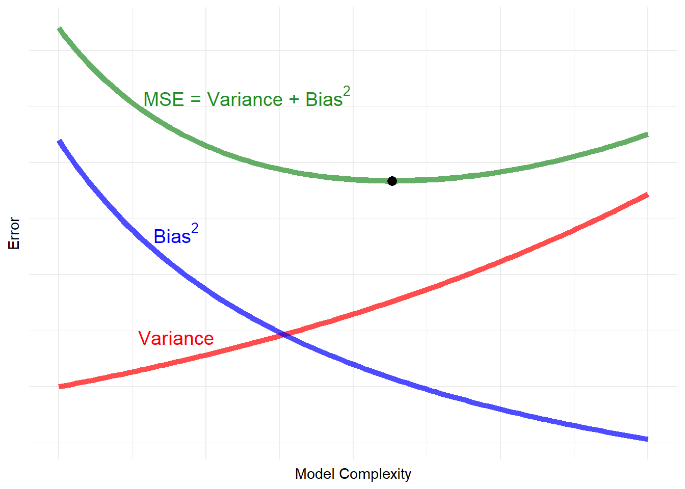
Figure 1: Traditional Bias-Variance Tradeoff
The double descent phenomenon, on the other hand, causes the U-shaped prediction error curve to decrease after a certain point. The variance starts to decrease as the model has more and more predictors (and parameters to estimate), and the bias is essentially zero.
library(tidyverse)

#Prediction error function (it is piecewise so creating two of them).
f1 <- function(x){
  ifelse(x<=2,   (-0.4 + 1/(x+0.5)) + (0.5*exp(x)), NA)
}

f2 <- function(x){
  ifelse(x>=2, (0 + 1/(1/(0.5*exp(4/x)))), NA)
}

#Prediction variance function (it is piecewise so creating two of them).
var_f1 <- function(x){
  ifelse(x<=2,   (0.5*exp(x)), NA)
}
var_f2 <- function(x){
  ifelse(x>=2, 1/(1/(0.5*exp(4/x))), NA)
}

#Prediction bias function (it is piecewise so creating two of them).
bias_f1 <- function(x){
  ifelse(x<=2,-0.4 + 1/(x+0.5),NA )
}
bias_f2 <- function(x){
  ifelse(x>=2,0,NA )
}

ggplot(data = temp_data, aes(x=x, y=y)) +
  xlim(0,4) +
  geom_function(fun = var_f1, color = "red", size = 2, alpha = 0.7) +
  geom_function(fun = var_f2, color = "red", size = 2, alpha = 0.7) +
  geom_function(fun = bias_f1, color = "blue", size = 2, alpha = 0.7)  +
  geom_function(fun = bias_f2, color = "blue", size = 2, alpha = 0.7)  +
  geom_function(fun = f1, color = "forestgreen", size = 2, alpha = 0.7) +
  geom_function(fun = f2, color = "forestgreen", size = 2, alpha = 0.7) +
  geom_vline(xintercept = 2, linetype = "dashed") +
  geom_point() +
  theme_minimal() + ylab("Error") + xlab("Number of Predictors/Number of observations") +
  theme(axis.text=element_blank(),
        axis.ticks=element_blank()) +
  annotate("text", x=0.32, y=-0.2+1/(0.2+0.5), label= expression(paste("B", ias^2)), color = "blue") +
  annotate("text", x=0.2, y=-0.2+0.5*exp(0.2), label= "Variance", color = "red") +
  annotate("text", x=0.26, y=0.21+(0.5*exp(0.2) + 1/(0.2+0.5)), label= expression(paste("Variance + B", ias^2)), color = "forestgreen") +
  annotate("text", x=2.4, y=-0.2+1/(0.2+0.5), label= "Interpolation limit", color = "black") +
  ggtitle("")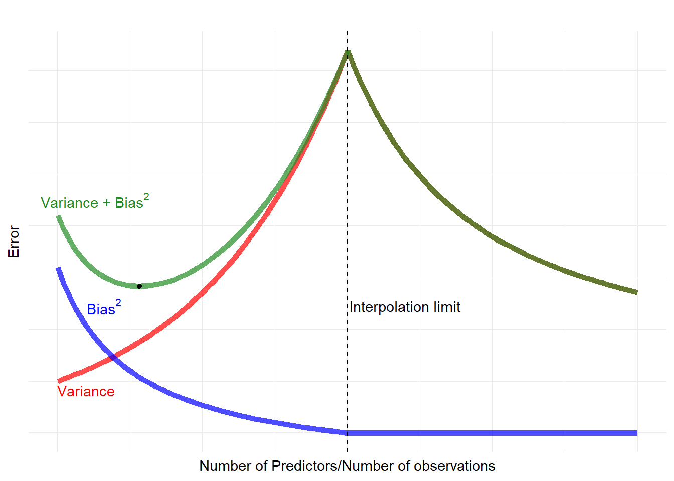
Figure 2: Double Descent
What just happened here? We hit the interpolation limit and reach the over-parameterized regime, and suddenly the variance started to decrease. How did this happen? Let’s clarify something before we move further: We changed the x-axis label. It is no longer “model complexity”, but the ratio of the number of predictors to the number of observations. Does it matter? Before the interpolation threshold, not so much. After the interpolation threshold, it does. It depends on how we define the term “complexity”. We may say that once we hit the interpolation limit, the complexity no longer increases, because the model is as complex as the training data allows. Or we can define complexity in terms of the \(\ell_{2}\) norm of the coefficient estimates (\((\mathbf{\beta^{T}\beta})^{1/2}\)). Then, in fact, as the ratio increases, the norm may decrease.2
Back to the main question: What just happened? We will examine this in more detail in later posts as well. Briefly, when the number of predictors is larger than the number of observations in the training sample, the estimator automatically regularizes itself. This happens even if we do not explicitly apply any of the regularization methods. The estimator becomes picky. Because there are more predictors (p) than the number of observations (n), it can focus on tasks other than minimizing the training error (which is usually 0 when \(n \leq p\)). One of those tasks can be minimizing the norm, which allows the estimator to prefer the most powerful predictors to others.
Samplewise Non-monotonicity
Usually, in the double descent literature, the focus is on the number of predictors. In particular, given the sample, whether the neural network should be wider or deeper is the main focus of attention. In this first part, however, we will hold the number of parameters constant and change the sample size. Since we are interested in the shape of the bias-variance trade-off curve and we have p/n in the x-axis, for our purposes, it matters little if n or p changes as long as p/n changes.
In this simple example, we consider the case where the underlying data generating process is as follows:
\[ y = \mathbf{X\beta} + \varepsilon \] with \(\mathbf{X}\) and \(y\) are known and \(\mathbf{\beta}\) and \(\varepsilon\) are unknown. Let’s say there are 100 known predictors (\(\mathbf{X}\) has 100 columns). The data is produced as follows:
num_predictor <- 100
create_data <- function(sigma, training_sample_size){
  X <- matrix(rnorm(10000*num_predictor), ncol = num_predictor)

  #Coefficients
  beta <- runif(num_predictor)
  beta <- beta/sqrt(sum(beta^2)) ## Normalizing so that the norm is 1

  #Error term
  e <- rnorm(10000, sd = sigma)
  #The outcome
  y <- X %*% beta + e

  X_train <- X[1:training_sample_size,]
  y_train <- y[1:training_sample_size, ,drop = FALSE]

  X_test <- X[(training_sample_size+1):nrow(X),]
  y_test <- y[(training_sample_size+1):nrow(y), ,drop = FALSE]

  return(list(y_train=y_train, X_train=X_train,
              y_test=y_test, X_test=X_test,
              e=e, beta=beta))

}
Linear Models
It is surprisingly straightforward to obtain the sample-wise double descent with the linear model. The trick is that when the number of observations is smaller than the number of predictors (i.e. after the interpolation limit where there are multiple solutions), one can use the Moore-Penrose inverse to calculate $ = $, as the \(\mathbf{(X^{T}X)^{-1}}\) part is undefined. Moore-Penrose inverse chooses the solution with the smallest Euclidean norm of the coefficients when there are multiple solutions. When the matrix is invertible and there is a unique solution, the Moore-Penrose inverse is numerically same as the regular inverse of the matrix. So we use it to obtain \(\widehat{\beta}\) for any p/n.
Based on Iyar Lin’s reproduction of the “More Data Can Hurt for Linear Regression: Sample-wise Double Descent” paper by Preetum Nakkiran, the following code produces two lines for two different data generating processes: one with no error term (\(\mathbf{y} = \mathbf{X*} \mathbf{\beta}\)) and another with normally distributed error term with mean 0, standard deviation 0.1 ($ y = + $).
library(furrr)  # For parallel processing
num_workers <- parallel::detectCores() - 1L

#Estimation
LS_estimator <- function(sigma = 0.1, training_sample_size = num_predictor){
  # Putting the number generators inside to obtan the exact same data every time.
  set.seed(5)
  full_data <- create_data(sigma=sigma, training_sample_size = training_sample_size)

  #Estimate coefficients with the training data and predict y_test
  beta_hat <- MASS::ginv(full_data$X_train) %*% full_data$y_train
  y_test_hat <- full_data$X_test %*% beta_hat

  #Return the RMSE for given sigma and sample size.
  data.frame(rmse = sqrt(mean((full_data$y_test - y_test_hat)^2)),
                     sigma = sigma,
                     training_sample_size = training_sample_size)

}

# We are saving the file to save time.
if (file.exists("all_results_lm.rds")) {
  res <- readRDS("all_results_lm.rds")
} else {
  plan(multisession, workers = num_workers)
  alternative_values <- expand.grid(
    sigma_values = c(0,0.1),
    training_sample_size_values = c(num_predictor*c(0.5, 0.75, 0.9, 0.95, 1, 1.05, 1.1, 1.25, 1.5))
  )
  res <- future_map2_dfr(.x = alternative_values$sigma_values,
                         .y = alternative_values$training_sample_size_values,
                         .f = ~LS_estimator(sigma = .x,
                                                  training_sample_size = .y),
                         .options = furrr_options(scheduling = 25, seed = FALSE))
  plan(sequential)
  saveRDS(res, "all_results_lm.rds")
}

#The plot
dd_plot <- ggplot(data = res) +
  geom_line(aes(x = training_sample_size, y= rmse, group = factor(sigma), color = factor(sigma)), size = 2) +
  geom_point(aes(x = training_sample_size, y= rmse, group = sigma, color = factor(sigma)), size = 3)  +
  theme_bw() +
  coord_cartesian(ylim = c(0, 1)) +ylab("RMSE") + xlab("Training Sample Size") +
  theme(text=element_text(size=15))

dd_plot$labels$colour <- "Std. Dev. of Error"

dd_plot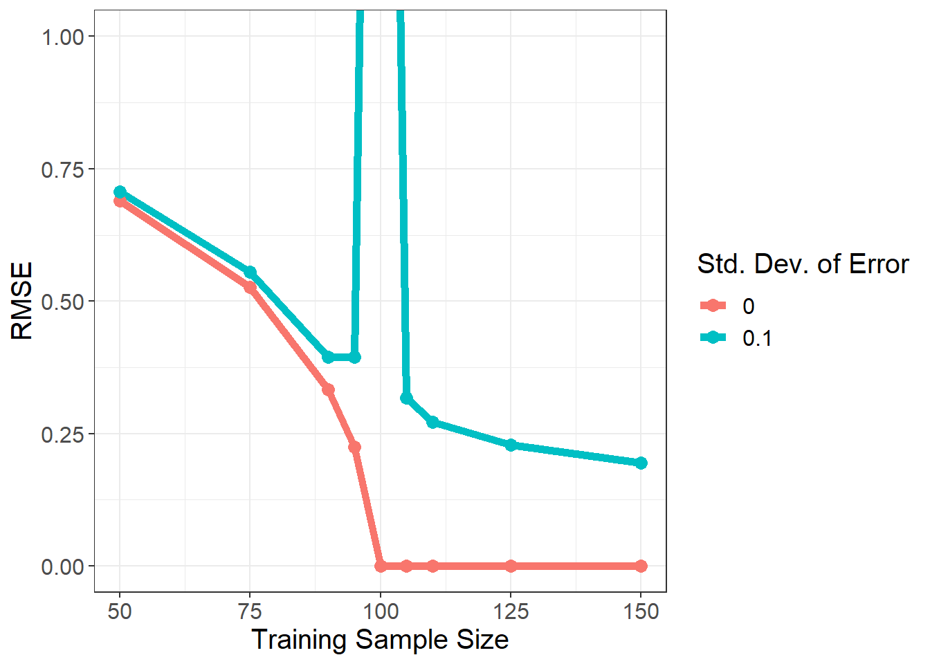
Figure 3: Samplewise Double Descent with Linear Estimator
Let’s start with the unsurprising curve, the red one. What happens is that as the training sample size increases (p/n decreases), the RMSE decreases. When the number of observations in the training sample size is 100, we have 100 unknown variables and 100 equations, and the system has a unique solution. As a result, the RMSE hits 0, and remains 0 thereafter.
Now, the surprising one curve, the turqoise colored line. In the beginning, everything is expected: more data brings more information and more information decreases the RMSE. But then, p/n is very close to 1, the RMSE suddenly shots up. It becomes so big that we have to cut the graph (the RMSE is more than 3 when p/n = 1). The error term completely confuses the estimator. However, the confusion only happens in the small neighborhood of p/n = 1, and the RMSE quickly decreases when the sample size increases.
Neural Networks
Another question is whether we see the same pattern with the neural networks. Note that the spike in the RMSE occurs when there is a unique set of coefficients that solves the system and there is irreducible error; namely pure noise. So, these coefficients are correct and they are the only ones that solve the system when \(p/n \leq 1\). Neural networks tend to use gradient descent methods to obtain the coefficients. These coefficients will be approximately correct. Let’s see how neural networks perform in the same scenarios.
library(torch)


NN_estimator <- function(sigma = 0.1, training_sample_size = num_predictor){
  # Putting the number generators inside to obtan the exact same data every time.
  set.seed(5)
  torch_manual_seed(5)

  full_data <- create_data(sigma=sigma, training_sample_size = training_sample_size)

  full_data$x_train_tensor = torch_tensor(full_data$X_train, dtype = torch_float())
  full_data$y_train_tensor = torch_tensor(full_data$y_train, dtype = torch_float())
  full_data$x_test_tensor = torch_tensor(full_data$X_test, dtype = torch_float())


  torch_dataset <- dataset(

    name = "my_data",

    initialize = function() {
      self$x_train <- full_data$x_train_tensor
      self$y_train <- full_data$y_train_tensor
    },

    .getitem = function(index) {

      x <- self$x_train[index, ]
      y <- self$y_train[index, ]

      list(x, y)
    },

    .length = function() {
      self$x_train$size()[[1]]
    }
  )

  train_ds <- torch_dataset()
  train_dl <- train_ds %>%
    dataloader(batch_size = 25, shuffle = FALSE)


  # Pretty basic 1-layer neural network model (mathematically identical to the least squares estimator)
  #Naturally, this is extremely inefficient way to do this, but let's use nn_linear.
  net = nn_module(
    "class_net",

    initialize = function(){

      self$linear1 = nn_linear(num_predictor,1)

    },

    forward = function(x){

      x %>%
        self$linear1()

    }

  )

  model = net()

  optimizer <- optim_adam(model$parameters)
  n_epochs <- 2000
  device <- "cpu"

  train_batch <- function(b) {

    optimizer$zero_grad()
    output <- model(b[[1]]$to(device = device))
    target <- b[[2]]$to(device = device)

    loss <- nnf_mse_loss(output, target)
    loss$backward()
    optimizer$step()

  }


  for (epoch in 1:n_epochs) {

    model$train()

    coro::loop(for (b in train_dl) {
      loss <-train_batch(b)
    })

    if (epoch %% 100 == 0 ){
     cat(sprintf("\nEpoch %d", epoch))
    }

  }


  model$eval()

  y_test_hat <- model(full_data$x_test_tensor)
  y_test_hat <- as_array(y_test_hat)


  #Return the RMSE for given sigma and sample size.
  data.frame(rmse = sqrt(mean((full_data$y_test - y_test_hat)^2)),
                     sigma = sigma,
                     training_sample_size = training_sample_size)

}


if (file.exists("all_results_nn.rds")) {
  res_nn <- readRDS("all_results_nn.rds")
} else {
  alternative_values <- expand.grid(
    sigma_values = c(0,0.1),
    training_sample_size_values = c(num_predictor*c(0.5, 0.75, 0.9, 0.95, 1, 1.05, 1.1, 1.25, 1.5))
  )
  res_nn <- data.frame()
  for (zz in c(1:nrow(alternative_values))){
      res_nn <- bind_rows(res_nn , NN_estimator(
        sigma = alternative_values$sigma_values[zz],
        training_sample_size = alternative_values$training_sample_size_values[zz]
      ))

  }


  saveRDS(res_nn, "all_results_nn.rds")
}

#The plot
dd_plot <- ggplot(data = res_nn) +
  geom_line(aes(x = training_sample_size, y= rmse, group = factor(sigma), color = factor(sigma)), size = 2) +
  geom_point(aes(x = training_sample_size, y= rmse, group = sigma, color = factor(sigma)), size = 3)  +
  theme_bw() +
  coord_cartesian(ylim = c(0, 1)) +ylab("RMSE") + xlab("Training Sample Size") +
  theme(text=element_text(size=15))

dd_plot$labels$colour <- "Std. Dev. of Error"

dd_plot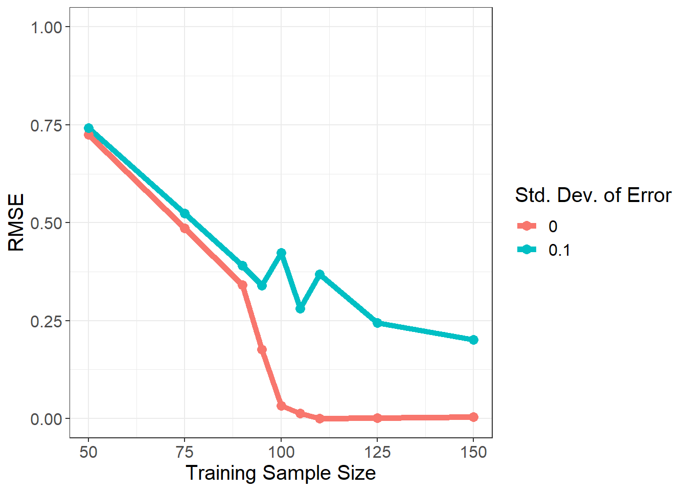
Figure 4: Samplewise Double Descent with Neural Network
Wow!!! The sample-wise double descent did not appear as strongly with the neural networks. This is really interesting. The optimization algorithm has avoided the spike around p/n = 1 (or training sample size = 100).
When the error term is non-existent (red curve), the neural networks did an OK job. The error is not 0 at p/n, which was the case for the linear model, but it was not too big either. But when the error term is non-negligible (turqoise curve), allowing some imperfections proved to be very helpful, especially if we are interested in preventing some catastrophic fails. There occurred some increase in RMSE at p/n = 1, but it is certainly not of the proportions that we have seen in the linear model graphs.
Cost of Perfection
We know that the correct coefficient estimates, the set of coefficients that provide the unique solution, come from the linear model and we know that neural network coefficients are, in this sense, approximately correct. By decreasing the learning rate (the size of steps towards the correct solution that the neural network takes) and trying out alternative number of epochs, let’s see at what point do we observe the cost of perfection when p/n = 1 and standard deviation of the error term is not 0. The expectation is that in the beginning, when the number of epochs is too small, the RMSE will be quite high because we would be quite far from the correct solution. As we increase the number of epochs, the RMSE will go down initially. After a certain point, it will go up again.
library(torch)


NN_estimator <- function(sigma = 0.1, training_sample_size = num_predictor, n_epochs){
# Putting the number generators inside to obtain the exact same data every time.
  set.seed(5)
  torch_manual_seed(5)

  full_data <- create_data(sigma=sigma, training_sample_size = training_sample_size)

  beta_hat <- MASS::ginv(full_data$X_train) %*% full_data$y_train
  y_test_hat_lm <- full_data$X_test %*% beta_hat
  y_train_hat_lm <- full_data$X_train %*% beta_hat


  full_data$x_train_tensor = torch_tensor(full_data$X_train, dtype = torch_float())
  full_data$y_train_tensor = torch_tensor(full_data$y_train, dtype = torch_float())
  full_data$x_test_tensor = torch_tensor(full_data$X_test, dtype = torch_float())


  torch_dataset <- dataset(

    name = "my_data",

    initialize = function() {
      self$x_train <- full_data$x_train_tensor
      self$y_train <- full_data$y_train_tensor
    },

    .getitem = function(index) {

      x <- self$x_train[index, ]
      y <- self$y_train[index, ]

      list(x, y)
    },

    .length = function() {
      self$x_train$size()[[1]]
    }
  )

  train_ds <- torch_dataset()
  train_dl <- train_ds %>%
    dataloader(batch_size = 25, shuffle = FALSE)


  # Pretty basic 1-layer neural network model (mathematically identical to the least squares estimator)
  #Naturally, this is extremely inefficient way to do this, but let's use nn_linear.
  net = nn_module(
    "class_net",

    initialize = function(){

      self$linear1 = nn_linear(num_predictor,1)

    },

    forward = function(x){

      x %>%
        self$linear1()

    }

  )

  model = net()

  optimizer <- optim_adam(model$parameters, lr = 1e-5)
  device <- "cpu"

  train_batch <- function(b) {

    optimizer$zero_grad()
    output <- model(b[[1]]$to(device = device))
    target <- b[[2]]$to(device = device)

    loss <- nnf_mse_loss(output, target)
    loss$backward()
    optimizer$step()
    loss$item()
  }


  final_data <- data.frame()
  for (epoch in 1:n_epochs) {

    model$train()
    train_loss <- c()
    coro::loop(for (b in train_dl) {
      loss <- train_batch(b)
      train_loss <- c(train_loss, loss)
    })
    model$eval()
    y_test_hat <- model(full_data$x_test_tensor)
    y_test_hat <- as_array(y_test_hat)

    final_data <- bind_rows(final_data, data.frame(rmse = sqrt(mean((full_data$y_test - y_test_hat)^2)),
           epoch = epoch,
           train_loss = mean(train_loss)))


    if (epoch %% 50 == 0 ){
      cat(sprintf("\nEpoch %d, training: loss: %3.5f \n", epoch, mean(train_loss)))
      cat(sprintf("\nTot Epoch num %d", n_epochs))
    }

  }


  #Return the RMSE for given sigma and sample size.
  final_data <- final_data %>%
    mutate(rmse_lm = sqrt(mean((full_data$y_test - y_test_hat_lm)^2))) %>%
    mutate(rmse_lm_training = sqrt(mean((full_data$y_train - y_train_hat_lm)^2)))


  return(final_data)

}


if (file.exists("cost_of_perfection_nn.rds")) {
  res_nn_cp <- readRDS("cost_of_perfection_nn.rds")
} else {
  res_nn_cp <- NN_estimator(
        n_epochs = 100000
      )


  saveRDS(res_nn_cp, "cost_of_perfection_nn.rds")
}

ggplot(data = res_nn_cp) +
  geom_line(aes(x=epoch, y = rmse, color = "Neural network"), size = 2) +
  geom_line(aes(x=epoch, y = rmse_lm, color = "Linear model"), size = 2) +
  theme_bw() +
  scale_color_manual(name = "Models",
                     values = c("Neural network" = "darkgreen",
                                "Linear model" = "red")) +
  ylab("RMSE") + xlab("Number of Epochs") +
  theme(text=element_text(size=15))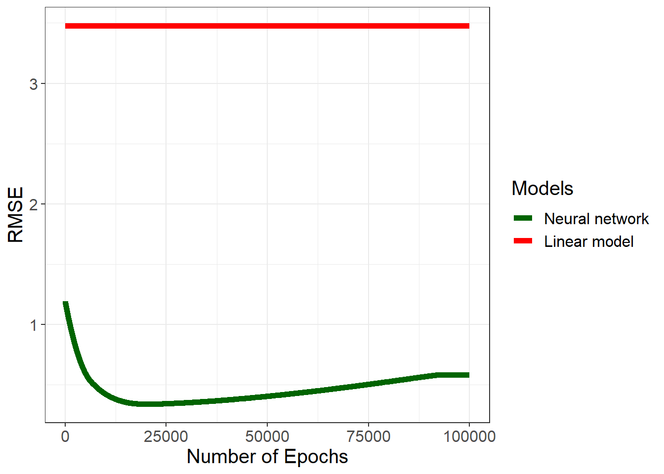
Figure 5: Cost of Perfection
We do see the expected U-shaped RMSE curve, but the latter half of it never reaches the levels that the linear model reaches. The cost of perfection (though calling it cost of approximate perfection would be more apt) is quite small in the case of neural networks. Since the gradient descent algorithm never really reaches the exact set of coefficients, it never really pays the full price of the perfectionism. This occurs even when we select a relatively small learning rate (\(10^{-5}\)) and many epochs (\(10^6\)), and we achieve a training error that is smaller than \(10^{-13}\).3 But the main point here is that the training error is not 0, so our solution is approximately correct for the training data. This has negligible effects for every p/n values other than 1. But when p/n = 1, the perfection vs. approximate perfection matters.
The general idea of allowing some imperfections to get better predictions should not be too novel, since the whole idea behind LASSO or Ridge regressions is to allow some bias to reduce variance. It is just nice to see how it can reveal itself under different scenarios. We will continue to see this pattern in the coming blog posts related to the double descent phenomenon as well.
In this example, we used MSE as the prediction error. Other accuracy metric would yield qualitatively similar results in the sense that the sweet spot minimizes neither the variance nor the bias.↩︎
This is shown in the paper titled “Triple descent and the Two Kinds of Overfitting: Where & Why do they Appear?” by d’Ascoli, Sagun, and Biroli.↩︎
If the learning rate was infinitely small and the number of epochs was infinitely large, then we would reach the linear model solution.↩︎